
Page 100 - IJEEE-2022-Vol18-ISSUE-1
P. 100
96 | Al-Flehawee & Al-Mayyahi
Where the battery power can also be expressed[17]: (14) model, which is a mathematical model that describes the
?????????? = ???????? + ???????? work of the plant, where the current measurements of the
plant at the moment of sampling, represented by the values
After substitute (13) into (14), we get:- of state variables and optimal inputs (MVs), are used to
predict the future behavior of the plant during a finite time
????? ?? = ??????-v??????2-4??????????(????????+ ???????? ) (15) interval called the prediction horizon. The prediction horizon
can be defined as the future in which the algorithm can see
- the future behavior of the plant. At each sampling time, this
2???????????????????? algorithm works to find a solution to the optimization
problem to obtain values of the optimal inputs trajectory,
From (1) we obtain:- where only the first value of this trajectory is applied to the
plant until the next sampling moment is reached. Because of
???? = ??3???? + ??3???? the formulation of this algorithm and its dependence on
Now substitute ???? into (15) process measurements at the moment of sampling to find the
optimal inputs trajectory, it is considered as an open-loop
????? ?? = - ??????-v??????2-4??????????(((???+? ??)????-????????)????+ ???????? ) (16) controller [20].
2???????????????????? Fig.4 shows the basic work of MPC, in which the MPC
algorithm, at each sampling step, re-solves the optimization
C. Fuel Flow Rate equation problem of open-loop control subject to system dynamics
and constraints. Where the measurements obtained from the
Through the experimental data of the fuel flow rate obtained process model at current sampling time are used by the MPC
algorithm to predict the future dynamics behavior of the
by (http://www.transportation.anl.gov/pdfs/HV/2.pdf), a plant y (•|k) over a prediction horizon ???? . Result of
optimization problem solving is getting the optimal control
mathematical relationship was formed between the fuel flow input trajectory u (•|k), where only the first value of this
trajectory is used to fed the next sampling step[21][22].
rate on the one hand, and on the other side, both speed and
torque generated by the engine, by applying the multiple
linear regression analysis method[18]. Where this method is
used to form a mathematical model between a dependent
variable represented here by the fuel flow rate, and several
independent variables represented here by both the speed and
torque generated by the engine, as shown in (17).
??? ?? = ?? + ?? ???? + ?? ???? (17)
Where the least square method is used to estimate
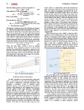
coefficients of the regression, ??, ??, ?????? ?? in (17). Fig.3
represents the mathematical relationship to express the fuel
flow rate in terms of both the rotational speed and the output
torque of the engine, and it is noted in this figure that when
the rotational speed and torque of the engine are increased,
the fuel flow rate increases linearly.
Fig.3: The fuel flow rate function Fig.4: Basic principle of MPC
Due to the large number of computations resulting from
IV. MODEL PREDICTIVE CONTROL predicting the behavior of system dynamics and solving the
optimization problem at each sampling step over the
The MPC algorithm is a process methodology (approach) prediction horizon, this definitely increases the demand for
used to control dynamic constrained systems[19], which is computation. The computational complexity can be greatly
well suited to multivariate constrained operations. This reduced by introducing a horizon called the control horizon
algorithm is considered a class of computer control ???? which is less than the prediction horizon. Where after the
algorithms because it iteratively solves the optimization time interval of the control horizon ???? , the output of the
problem of this algorithm at each sampling step in order to controller is constant, where the value of the output of the
find the optimal control input trajectory (manipulated controller is the value of the optimal control input at the
variables (MVs)) of the plant. To achieve the control sampling step of the control horizon ????, assuming that the
objectives on which this algorithm is built, it is formulated in system has reached the steady-state[23], as shown in Fig.4.
the form of an optimization problem, which includes the cost If the predictions of the dynamic behavior of the plant
function, which represents the objectives to be achieved by are obtained from the equations of the nonlinear model, then
the algorithm, where the cost function is subject to the MPC in this case is called the Nonlinear Model Predictive
predictions of the future behavior of the plant in addition to Control (NMPC). Therefore, nonlinear predictive model
the plant's physical constraints. The predictions of the future control is an extension of linear predictive control
behavior of the plant are obtained when using a process