Page 219 - 2024-Vol20-Issue2

215 | Gochhait, Sharma & Bachute

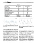
TABLE IX.
COMPARISON OF LONG-TERM ELECTRICITY FORECASTING ANALYSIS

Aspect Orissa Delhi
Training Options Adam optimization Adam optimization
Gradient Threshold
Initial Learning Rate 1 N/A
Maximum Epochs 0.001 N/A
Evaluation Metric N/A
Average RMSE (6 months) 10 RMSE
Frequency RMSE 0.864
Dataset Duration 0.952 Day wise
Data Cleaning and Transformation Hourly 2 years
Data Reduction Techniques 5 years Yes
Forecasted Response Yes
Training Set Size Yes Load Demand (MW) for 9 months
Validation Set Size Yes 70% (997 rows)
Testing Set Size Load Demand (MW) for 12 months 10% (142 rows)
70% (1,273 rows) 20% (285 rows)
10% (181 rows)
20% (363 rows)

Fig. 2. Graph of actual versus predicted load for the Odisha Fig. 3. Graph of actual versus predicted load for the Delhi
state over six months (March 2022 to August 2022) using 1D State over six months (March 2022 to August 2022) using 1D
CNN BI LSTM. CNN BI LSTM.

networks provides superior performance compared to using Odisha State overa six-month period (March 2022 to August
either CNNs or LSTMs alone. For the case study of Orissa 2022) using the 1D CNN-BI LSTM model.The model demon-
state, the CNN-BI LSTM hybrid model with deep1D mod- strates accurate load forecasting for the given timeframe. For
eling was used. The model architecture consists of multiple the case study of Delhi state, a similar CNN-BI LSTM hybrid
layers, including sequence input layer, convolutional layers model was used with a slightly different configuration. The
with different filter sizes, batch normalization layers, recti- model architecture and training optionsfor the Delhi state are
fied linear unit (ReLU) layers, dropout layers ,bidirectional provided in Table VII and Table VIII, respectively.
LSTM layers, fully connected layer, and regression layer. The
complete configuration details are presented in Table V. The In conclusion, the comparative long-term electricity fore-
training options used for the Orissa state include parameters casting analysis of Orissa and Delhi states demonstrates the
such as gradient threshold, initial learning rate, maximum effectiveness of the hybrid 1D CNN-BI LSTM model in accu-
epochs, sequence length, epsilon, L2 regularization, shuffle, rately predicting peak load values. The model’s architecture
gradient decay factor, squared gradient decay factor, learning and training options, along with the obtained results, provide
rate drop factor, learning rate drop period, gradient threshold valuable insights for future research and practical applications
method, reset input normal- ization, and training plots. The in the field of electricity forecasting. Fig. 3 depicts the graph
specific values for these options are provided in Table VI. of actual versus predicted load for the Delhi State over the
Fig. 2 shows the graph of actual versus predicted load for the same six-month period using the CNN-BI LSTM model. The