Page 100 - 2023-Vol19-Issue2

96 | Al-Ansarry, Al-Darraji & Honi

O(|E| + |V |log|V |), where E is the set of edges and V
is the set of vertices. On the other hand, A* has a worst-
case time complexity of O(bdˆ), where b is the branching
factor of the graph and d is the depth of the optimal
solution. However, in practice, A* often performs better
than Dijkstra due to its use of the heuristic function.

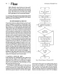
As a conclusion, the proposed dynamic path planning method
(Dynamic D-PF) can be illustrated through the blocks diagram.
Figure (6), shows the steps clearly.

III. EXPERIMENTAL RESULTS

The proposed method was evaluated through a series of experi-
ments in a simulated 2D environment. The performance of the
(Dynamic D-PF) was evaluated in terms of path length, safety,
and execution time. The path length was measured as the total
distance traveled by the robot starting from the initial location
to the target one. The safety of the path was evaluated by the
number of times the robot encountered a dynamic obstacle
and had to switch to a different path. The execution time was
measured as the time it took for the robot to complete the path
from start to finish. A variety of scenarios were tested, with
different numbers and types of static and dynamic obstacles,
and different levels of complexity in the environment. The
start point depicts as an orange circle and the goal point as a
green circle. The shortest global path (Dijkstra modified-path)
is represented by the red solid line. The dynamic real-time
path (generated by PF) is shown by the solid green line and
the final resulting path (generated by Dynamic D-PF) is repre-
sented by a black dotted line, which is calculated based on the
proposed method. The grey dotted line represents the desired
path-net, generated using the (Dijkstra algorithm) to cover
most free configurations. Static obstacles are denoted by black
blocks, while dynamic obstacles are represented by blue wide
arrows. Finally, the robot is acted by a blue polygon. The
simulation is built using Lenovo intel Core i7 8Gen laptop
with a Linux 20.04, Python-3 under the Robotic Operating
System (ROS) framework, and Rviz environment.

A. Experiment-1: (Global Path - Static) Fig. 6. Blocks Diagram of Dynamic D-PF
In this experiment, the comparisons have been conducted by
implementing (A*, Dijkstra, and the Dijkstra-PF) on a static has to explore all the regions’ free obstacles which cause to
offline map of size (300*150 cm) for (100 runs). The planner increase the cost compare to A*. The Dijkstra-PF method
efficiency as the experimental results illustrated in Table I works to explore the desirable regions that have acceptable
below, is measured based on the time-consuming, cost, and costs. Moreover, in this experiment, the behavior that the
path length until reaching the goal. potential field takes influences the resulting path making it
shorter and smoother compared to that of A* and Dijkstra
The simulation results illustrate that the time and cost
consuming of A* is less than both Dijkstra and Dijkstra-PF
(D-PF) respectively, due to exploring the only regions with
minimum cost based on the heuristic function, while it cannot
deal with the dynamic obstacles. On the other side, Dijkstra