Page 97 - 2023-Vol19-Issue2

93 | Al-Ansarry, Al-Darraji & Honi

neighbor. If this new distance ¡ current distance to the potential field, allowing the robot to switch toward another
neighbor, the distances and previous dictionaries are path while still avoiding obstacles safely and efficiently. The
updated accordingly. proposed method operates in real-time and can handle mov-
able obstacles, making it suitable for use in a wide range of
• The previous dictionary and the distance starting from applications. The method is designed to find a path that is
the source node to the end one is returned as the result both short and safe, while also allowing the robot to react the
of the algorithm. variations in the environment and adjust its path accordingly.
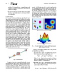
Figure (4) demonstrates the representation of the Artificial
B. Path Selection Potential Fields (APF).
The Potential Fields is a path planning algorithm that calcu-
lates a path between the start and goal positions while avoiding Fig. 4. Potential Fields Representation (a) 3D Environment
collisions that may occur in the environment. The algorithm (b) 2D Field (c) 3D Field
starts by initializing the current position to the start point and
runs a loop with a maximum amount of iterations. In each
iteration, the attractive force vector is calculated depending
on the current position and the goal location, while the re-
pulsive force vector is calculated depending on the current
location and the obstacles in the configuration. The vector of
the total-force is then calculated by adding the attractive and
repulsive force vectors and the current position is updated by
moving a small step in the direction of the total-force vector.
The distance between the current location and goal one is
checked, and if it is below a predefined threshold, a path to
the goal has been found and the algorithm returns the path. If
the maximum number of iterations is reached and no path is
found, the algorithm returns ”No path found”. In this phase,
the algorithm of the Potential Field (PF) is used to evaluate
the safety of each path generated by the Dijkstra algorithm.
The algorithm creates potential fields, where the gradient of
these fields as shown in Figure (3) guides the robot away
from obstacles and toward the goal point. The virtual path
represents by black dashed line and the actual path represents
by green dashed line. The attractive forces act as blue rows,
while repulsive forces as red rows.

The main mathematical equations used in the potential
field algorithm are as follows:

1. Attractive Force Vector Calculation: The attractive
force vector is calculated using Equation (1):

F attr = k attr * (goal - currentPos) (1)

Fig. 3. Potential Field Where: F attr: Attractive force vector, k attr: Attrac-
tive force constant (positive scalar value), goal: Goal
The safety of each path is evaluated based on the potential position, currentPos: Current position.
field, and the path with the safety highest score is chosen as
the optimal path. Additionally, the proposed method generates 2. Repulsive Force Vector Calculation: The repulsive
connections between the paths, allowing the robot to switch force vector is calculated using Equation (2) and (3) for
to different paths if it encounters a dynamic obstacle in its each obstacle in the environment:
current position. The connections are generated based on the
F rep = k rep * (1/distance - 1/d0) * direction (2)