
Page 98 - 2023-Vol19-Issue2
P. 98
94 | Al-Ansarry, Al-Darraji & Honi
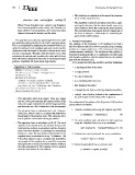
direction = (obs - curPos)/||obs - curPos|| (3) • The total force is calculated as the sum of the attractive
force and the repulsive force.
Where: F rep: Repulsive force vector, k rep: Repulsive
force constant (positive scalar value), obs: Obstacle, po- • The algorithm returns the normalized total force, repre-
sition curtPos: Current position, d0: Desired minimum senting the direction that the robot should move in to
distance between the obstacle and the robot. avoid obstacles while still reaching the target position.
The normalization step ensures that the magnitude of
The goal here is to select the optimal path from the multi- the force is always 1, which helps in controlling the
ple candidate paths generated in the Path Generation phase. speed of the robot’s motion.
This is accomplished by employing the Potential Field to cal-
culate the safety of each candidate path and combining this C. Problem Formulation
information with the length of the path to determine the over- The problem of the (Dynamic D-PF) method is to find a
all cost of each path. The path with the lowest cost is then safe and efficient path for a robot to navigate from a starting
selected as the optimal path, providing the robot with the best position to a target position in a 2D environment that may
trade-off between safety and efficiency in reaching the target contain dynamic obstacles. The solution to this problem is
position. Algorithm (2) shows these steps clearly. formulated mathematically as a combination of path length
and obstacle avoidance, and the method returns the optimal
path with the minimum cost.
Let’s assume the following variables and their definitions:
• s: starting position of the robot.
• t: target position.
• O: a set of obstacles.
• p: a candidate path from s to t.
• l(p): length of the path p.
• f obs(p): the rep force exerted by obstacles on path p.
• This algorithm, takes three inputs: robot pos, target, • cost(p): cost of path p, defined as the combination of
and obs. robot pos represents the current position of the the path length and the safety of the trajectory.
robot, the target represents the desired target position,
and obstacles are a list of obstacles in the environment. The mathematical formulation of the (Dynamic D-PF) method
can be defined as follows:
• The attractive force is calculated as k attr * (target -
robot pos), where k attr is a constant that determines 1. Generate candidate paths using the Dijkstra algorithm:
the strength of the attractive force. The attractive force
acts to pull the robot toward the target position. p candidates = Di jkstra(s,t) (4)
• The repulsive force is initialized as [0, 0]. For each 2. For each candidate path, calculate the safe trajectory
obstacle in the obstacles list, the distance between the using the Potential Field, for p in p candidates:
robot and the obstacle is calculated, and the direction
away from the obstacle is calculated as normalized sa f e tra jectory = PotentialField(s, p, O) (5)
(robot pos - obs). The contribution of the obstacle to the
repulsive force is calculated as k rep * (1/distance - d0) 3. Evaluate the cost of each path: for p in p candidates:
* direction, where k rep is a constant that determines
the strength of the repulsive force, and d0 is a constant cost(p) = l(p) + f obs(p) (6)
that represents a desired minimum distance between
the robot and obstacles. The repulsive force is updated 4. Select the path which has a minimum cost: (7)
with the contribution of each obstacle. p optimal = argmin pcost(p)