Page 255 - 2024-Vol20-Issue2
P. 255
251 |                                                                                        Sabeeh & Al-Furati

• Consideration of motion constraints: The robot’s
  motion is subject to specific constraints, such as maxi-
  mum velocity, acceleration, and turning radius. These
  constraints must be taken into account when planning
  the robot’s path, ensuring that the path adheres to the
  robot’s physical limitations.

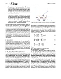
• Optimization of the path: The goal of the path-planning        Fig. 3. Illustrated example of a path-planning robot diagram.
  algorithm is to find an optimal path, which is a path
  that minimizes the total distance traveled from the start
  point to the goal point while avoiding collisions with
  all obstacles. The path-planning algorithm may use
  a variety of techniques to optimize the path, such as
  genetic algorithms or probabilistic roadmaps.

The initial positions of the dynamic obstacles are randomly      like navigation, self-localization, and object manipulation,
generated within the workspace. The number of dynamic            serving as the foundation for algorithms that empower robots
obstacles is determined is set to 50 in our code. This means     to reach specific destinations, evade collisions, and execute
that when we run the simulation, 50 dynamic obstacles will       tasks with precision and efficiency. In the proposed robot
be randomly placed within the workspace at the beginning         kinematics model, a differential drive robot with odometry
of the simulation. On the other hand, the speed of dynamic       updates is considered. The robot’s motion can be described
obstacles is set to 0.3 in the code, which represents the maxi-  using equations (1) to (3):
mum velocity that dynamic obstacles can have. The velocity
for each obstacle is randomly selected from the range of 0       dx = r  dfL + dfR  cos(? )  (1)
to velocitymax/2. This randomization adds variability to the     dt 2     dt dt
dynamic obstacle movement, making their speed dynamic and
unpredictable.                                                   dy r    dfL + dfR  sin(? )  (2)
                                                                     =    dt dt
B. System Model
In this section, we examine the use of a two-wheel differ-       dt 2
ential mobile robot for path planning. This particular robot
possesses the ability to control the speed of its two driving    d? = r dfR - dfL            (3)
wheels, granting it the flexibility to execute a range of tra-   dt 2L dt dt
jectory movements, such as moving in straight lines, making
turns, and performing circular maneuvers. We establish a         Where:
kinematic model by tracking the robot’s consecutive positions,   (x, y): Robot coordinates in the global frame.
as illustrated in Figure 3.                                      ? : Orientation angle of the robot.
                                                                 r : Wheel radius L : Wheelbase (distance between the wheels).
1) The Motion Model of Mobile Robotic System                     dfL/dt, dfR/dt: Angular velocities of the left and right wheels.
In the field of mobile robotics, kinematics plays a pivotal
role in comprehending how a robot’s mechanical components,           Equations (1) to (3) represent the kinematic equations
such as wheels, sensors, and DC motors, operate and posi-        for the motion of a differential-drive mobile robot. These
tion themselves within their environment. It provides insights   equations describe how the robot’s position and orientation
into how a robot interacts with its surroundings and is indis-   change over time based on the angular velocities of its left
pensable for various tasks, including path planning, obstacle    and right wheels.
avoidance, and robot control. Kinematics enables engineers
and researchers to establish precise models of a robot’s be-         It is worth noting that the orientation angle of the robot
havior and make predictions about its actions in diverse sce-    gives the direction in which the robot is pointed. Typically, ?
narios. Leveraging mathematical and geometrical principles,      is measured relative to some reference, such as the positive
kinematic models are formulated to illustrate the relationship   x-axis. For example, if ? is 0 degrees, the robot is facing
between the robot’s movements and the commands it receives.      directly along the positive x-axis. If ? is 90 degrees, the robot
Moreover, robot kinematics proves vital for exacting tasks       is facing along the positive y-axis. If ? is 180 degrees, the
                                                                 robot is facing directly along the negative x-axis, and so on.
                                                                 In addition, the velocity variables in Equation (3) are crucial

