Page 53 - 2023-Vol19-Issue2

49 | Hashim & Yassin

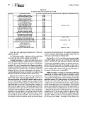
TABLE III.
PC-MI METHOD FOR FEATURE SELECTION

groups Correlated features Pearson Correlation Score chosen feature of a high mutual information value
[ radius mean,area worst] 0.947
1 [ radius mean,perimeter worst] 0.967 perimeter worst
[ radius mean,radius worst] 0.971
2 [ radius mean,area mean] 0.989 texture worst
3 [ radius mean,perimeter mean] 0.998 concave points mean
4 [ area mean,area worst] 0.962
5 [ area mean,perimeter worst] 0.961 area se
[ area mean,radius worst] 0.965 concavity worst
[ radius worst,area worst] 0.986
[ radius worst,perimeter worst] 0.994
[ perimeter worst,area worst] 0.980
[ perimeter mean,area worst] 0.947
[ perimeter mean,perimeter worst] 0.972
[ perimeter mean,radius worst] 0.970
[ perimeter mean,area mean] 0.988
[ texture mean,texture worst] 0.907
[ compactness mean,concavity mean] 0.892
[ concavity mean,concave points mean] 0.930
[concave points mean,concave points worst] 0.913
0.956
[ radius se,area se] 0.970
[ radius se,perimeter se] 0.938
[ perimeter se,area se] 0.896
[ compactness worst,concavity worst]

•train–test–split (training=0.8,testing=0.2) k–fold cross involved in the classification job. This approach is appealing
validation (k=10) because, compared with learning a nonlinear surface, the cost
of moving to kernel space is minimal [24].
2) Classification Models: In this part, the ML models that
are used in this study will be explained and clarified. Decision Tree: A DT is one of the most important models
in decision-making processes, as it is widely used in the field
Logistic Regression: A statistical model known as LR of ML. The trees are built from top to bottom, and nodes
uses a qualitative dependent variable that can only use discrete of these trees representing features are selected based on a
values to represent the connection between two independent certain scale (information gain in this study). In each node of
variables. It is used to investigate the influence of predictor the tree, a specific decision is made, and this decision directs
variables on categorical outcomes. In an epidemiologic study, you to another level of the tree until the root node, which is
logistic models are frequently used to analyse the connections the source of the decision, is reached[25].
between risk factors and the development of the disease. In
medical publications that do not specialize in epidemiology Voting Classifier: It is a type of ensemble classifier that
and public health, these models are often utilised [23]. depends on AI models, where it works to combine a certain
set of models to produce one model that carries the strength
Support Vector Machine: When learning the parameters of the models that have been combined, which gives the best
of the SVM model during the training phase, SVM, one of prediction accuracy [26]. Here, we use a soft voting classifier
the most significant and potent ML models, needs access to and input three ML models (LR, SVM and DT), which are
all of the training data. Support vectors, a subset of these considered the best models that work with a voting classifier
training examples, are the only ones on which SVM relies to on this dataset based on a set of experiments. This classifier
make predictions in the future. The hyperplanes’ margins are works on a probabilistic basis, as each of the input models of
determined by support vectors. Finding the greatest number the classifier produces a probability value for class 0 and class
of hyperplanes that may be used to divide two classes is the 1. In the final result, the soft voting classifier uses the highest
major goal of the training phase. When an issue is not linearly probability rate of all the input models, as shown in Fig.6.
separable in the input space, a kernel can transfer the data Finally, we can summarize the proposed methodology as the
into a higher-dimensional space called kernel space, where following. Firstly, we carry out some preliminary treatments
the data will be linearly separable. Linear hyperplane can for improving the dataset. Secondly, the best features are
be obtained in the kernel space to divide the several classes