
Page 50 - 2023-Vol19-Issue2
P. 50
46 | Hashim & Yassin
dataset performs two main processes as follows. Firstly, the SMOTE balances the dataset between majority and minority
number of features that are actually used is only 30. As the classes.
dataset consists of 32 features, it involves two unimportant
features: ‘id’, and ‘Unnamed:32’, where ‘id’ is simply an 3) Label Encoder: In this stage, after performing the bal-
identifier and ‘Unnamed:32’ is a column whose rows are all ancing of the dataset, we will encode the target class ‘diag-
empty values, so we will drop this feature. Secondly, when nosis’ via transformation (Malignant to 1 and Benign to 0).
most of the values for each column or row are missing, we In classification analysis, the dependent variable is usually
drop that row or column to ensure the quality and correctness affected by qualitative factors and ratio scale variables. Hence,
of the data. In another case, if some column or row values are these category variables must be encoded into numerical val-
missing, the mean will be calculated to restore data. ues using encoding techniques because ML algorithms only
accept numerical inputs [17]. Fig. 3 shows the result of the
2) Balancing Dataset: The importance of a balanced label encoder on the diagnosis field in the dataset.
dataset for a model is to generate higher accuracy models
devoid of bias. Thus, a balanced dataset is important for a clas- (a) Without using label encoder
sification model. An uneven class distribution of the dataset
may cause trouble in later phases of training and classification
as classifiers will have very fewer data to learn features of a
particular class. SMOTE is one of the best techniques used
to balance the dataset. Unlike normal upsampling, SMOTE
makes use of the nearest neighbour algorithm to generate new
and synthetic data that can be used to train the models. It will
generate new data points for the minority class (in this case,
for class M) to balance the dataset where SMOTE gives the
minority class an increased likelihood of being successfully
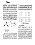
learned. Fig. 2 shows how to create new data by SMOTE[16].
(b) Using label encoder
Fig. 3. Label encoder on the dataset
Fig. 2. Smote technique [16]. B. Feature Selection Phase
In the beginning, and before choosing the model that fits
Fig. 2 shows two classes in the dataset: minority and
majority. The SMOTE technique works by using the nearest with our dataset, we should choose the appropriate features
neighbour algorithm to create new data points for the minority that our model will train on to yield the best results. Less
class located on the line connecting two data points of the redundant data means greater modeling accuracy, less mis-
same class represented by (a, b, c, d, e). The main benefit of leading data means fewer opportunities for decisions based
this process is the elimination of innate inclinations to favour on noise and less data equals faster algorithms. As a result,
and overfit toward the majority classes due to the disparity in the main objective of feature selection is to improve accu-
samples’ proportions of minority and majority classes. Finally, racy, reduce training time and decrease over-fitting [18]. In
this phase, we present a proposed method that combines two
methods from the filter method, which is correlation analysis
using Pearson correlation and mutual information. In the first
stage, we analyse the relationships in the dataset by finding
the correlation matrix that uses Pearson correlation as a mea-
sure and then we collect the highly correlated features that
contain common elements in one set. Our processing keeps
the common feature with the highest value mutual information
and drops the rest of the features in each group.
1) Correlation Analysis Based on Pearson Correlation:
Pearson Correlation (PC) is a measure of the degree of rela-