Page 106 - IJEEE-2023-Vol19-ISSUE-1

102 |
ball detecting leaks within the pipeline using acoustic
signals. With this information, trained guesses can be made
about where the leak is and how fast it is spreading. The
velocity, pressure, and temperature profiles will be used to
calibrate the internal control system using the Support
Vector Machine (SVM) and Decision Tree (DT) algorithms
for classification leaks using the ball. The control system
factors in the disruptions brought about by the fluid flow
around the ball, and it makes a relationship between the
levels of sound pressure and the detection of leaks.
Machine learning is a branch of artificial intelligence (AI)
and computer science that focuses on using data and
algorithms to imitate how humans learn, to constantly
improve the simulation's accuracy. Several kinds of machine
learning algorithms are often employed. These are as
follows: Support Vector Machine (SVM), Decision trees
(DT), and K- Nearest-Neighbor (KNN). This paper uses
SVM and DT for comparison. The obtained data of velocity,
pressure, and temperature distribution parameters, where the
leakage sound energy is applied, are employed within the
linear regression algorithm using SVM[27]. The detailed
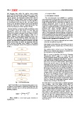
steps for developing the current SVM system are illustrated
in Fig. 1,
Fig. 1: SVM detailed steps.
MATLAB R2021a is used throughout this study to carry
out Support Vector Machine calculations (SVM) where the
optimum correction curve is utilized statistically using the
following Equation:
!"#$ = '?"($%"&'($)!(*., (1)
Where RMSE is a root mean square deviation of
resultant error.
Abed, Wali, & Alaziz
y: is response values
n: is the number of data set.
The root-mean-square error (RMSE) is a popularly
used measurement of the gaps that exist between the values
(both sample and population values) that are forecasted by a
model or estimator and the values that are observed. The
resultant optimization model is used for measurement
modification. When explaining or summarizing the expected
results of a classification problem, confusion matrices are a
beneficial tool. Linear regression algorithm develops
Support Vector machine prevails Confusion matrix. A
Confusion matrix's most crucial function is to provide a
class-by-class breakdown of the total number of correct and
incorrect guesses that have been generated. The performance
of the machine learning method can be investigated using the
parameters of precisions, accuracy, recall, and F1-score. The
confusion matrix determines the following [28], [29]:
- True Positive (TP): Both the value that was seen and the
value that was predicted are positive.
- False Negative (FN): When the actual observed value is
interpreted as having a negative sign, even when it has a
positive one.4
- The condition that is referred to as a “True Negative”
(TN) is one in which the observations are consistent with
the expectations of the null hypothesis.
When it comes to classifiers, the Receiver Operating
Characteristic (ROC) graph is a useful tool for
determining which element is the most essential. The rate
of true positives is represented along the ROC curve’s Y
axis, while the rate of false positives is shown along the
ROC curve’s X axis. The “ideal” location, which may be
found at the top left corner of the map, has a failure
probability of zero and a success probability of one. It is
evident that this is not the case; nevertheless, it does show
that a larger Area under the curve (AUC) is desirable in
the majority of circumstances [30], [31]. The “steepness”
of ROC curves is one factor that may affect the ideal
strategy, which is to increase the TP rate while decreasing
the FP rate. The analytical result was negative, but the
projection is that it will be positive. ROC curves are
frequently used for binary classification to evaluate the
output of a classification, and this is exactly what is being
done here because the classification technique includes
whether or not a leakage is identified [31].
The SVM and DT were trained using our dataset generated
from simulation, with extra leakage points added for
optimum performance during training and testing. The data
is divided using cross-validation (K-fold) with K=10, with
70% of the data randomly selected for training and 30% for
testing, with the accuracy evaluated at each iteration. The
data consist of three parameters (velocity, pressure, and
temperature). Each parameter has velocity values (0.1 m/s, 1
m/s, and 2.5 m/s). The confusion matrices of SVM after
training and testing the data is shown in Fig. 2, and the
confusion matrices of DT for training and testing data is
shown in Fig. 3,