Page 65 - IJEEE-2022-Vol18-ISSUE-1

Hussein & Ali | 61

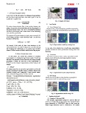
FL = -aC(1 - y^i)y. log y^i (2) Fig. 5: Sample of Dataset
B. Loss Results
? IoU Loss (Jacquard index)
1) Cross Entropy Loss
Loss of IoU It is the last option for unbalanced segmentation As you can see, cross-entropy has a problem segmenting
and has fewer hyperparameters than other types. It can be small areas and has the worst performance among these loss
explained in equation (3). functions.

IOU = Area of overlap (3) Fig. 6: Segmentation results by entropy loss.
As we note, cross-entropy has a small-space segmentation
Areaof Union problem and has the worst performance among these loss
functions.
The above shows that the filter is the overlap between the
masks of expected and ground truth, and the denominator is 2) Focal loss
the union between them. The IoU is calculated by dividing Focal loss can achieve better results, especially in small
the first by the second, with values closer to one indicating regions, but it still needs some hyper parameter tuning
more accurate predictions. through trial and error.

The purpose of the optimization is to get a more accurate IoU Fig. 7: Segmentation results using Focal loss
of the image and has a value between 0 and 1, so the loss 3) IOU (Loss)
function is defined as: Finally, we can see that IoU loss also does a great job in
segmentation, both for small and large areas.
IOU Loss = 1 - IOU (4)
Fig. 8: Segmentation results using IOU
We trained U-Net with all three loss functions of the C. Training the Model
mentioned data set. As only 65 images were used for training
and 7 images for verification, so we cannot expect perfect 1) Compare U-Net and CNN
results. But this number of data is sufficient for the purpose. The semantic segmentation purpose is used to label all
pixels in an image with an appropriate class. Original U-Net
V. RESULTS AND ANALYSES paper dimension is 572X572X3. Here in this work the
initial image dimension used is 128X128X3. All models
In this paper, we review the problem of semantic
segmentation on unbalanced type binary masks. Focal loss
and mIoU are presented as loss functions for tuning network
parameters. Finally, we train the U-Net implemented in
PyTorch on the semantic segmentation method using aerial
images.

A. Dataset

The dataset used here is a semantic segmentation set of aerial
images containing 72 satellite images of Dubai, United Arab
Emirates, divided into 6 categories. Classes include water,
land, roads, buildings, plants, and the unnamed.
filename = "/content/drive/MyDrive/semantic segmentation
dataset/classes.json"

shutil.unpack_archive(filename, extract_dir, archive_format)
self.BGR_classes = {'Water' : [ 41, 169, 226],
'Land' : [246, 41, 132],
'Road' : [228, 193, 110],
'Building' : [152, 16, 60],
'Vegetation' : [ 58, 221, 254],
'Unlabeled' : [155, 155, 155]} # in BGR
self.bin_classes = ['Water','Land','Road','Building','Vegetati

on', 'Unlabeled']